In accordance with ISO 80000-2, the following font conventions are employed:
Scalars and components for vectors or tensors are represented by lightface italic type ().
Vectors are represented by boldface italic type ().
Second-order tensors are represented by boldface sans-serif type ().
Operators & Constants: Roman (upright) type is used for fixed mathematical constants (e.g., Pi , the imaginary unit ) and differential operators (e.g., the differential in ).
Calculus Notation: For integrals, a thin space (\,) is used to separate the integrand from the differential operator, e.g., .
Minkowski Metric: The Minkowski metric tensor is defined using the mostly-plus signature convention:
Consequently, the invariant spacetime interval is given by .
Lorentz transformation
For -axis boost (where moves with velocity relative to ), the transformation matrix is:
1 Preparatory Math.
1.1 Vector and tensor analysis (Euclidean geometry)
1.1.1 Basics
Kronecker & Levi-Civita symbols
Determinant
Contraction identities
More generally*
and for high-dimensional case, we have generalized Kronecker delta
Axial Vector / Pseudovector
Symmetric-Antisymmetric decomposition
Double Contraction (adopt to the proximity rule)
1.1.2 Cross & dot product
Scalar Triple product
Vector Triple product / BAC-CAB formula
Lagrange's identity
Associative Law (the tensor remains centered in the contraction)
Cross Dot
1.1.3
Differential operations
Coordinate Component Expansion of Differential Operators
Two critical identities
Leibniz Rule
Taylor Series in Operator Form
Here, the terms in the parentheses are
is so-called "Translation Operator" in quantum mechanics or lie group ().
Integral operations
Coordinate-independent definition
Fundamental theorem of gradients
Generalized Gauss's Theorem
In Gauss's Divergence Theorem , if , one finds the Green's first identity:
and substituting yields the Green's second identity:
Generalized Stokes' Theorem
Helmholtz decomposition
For any continuous differentiable vector field , if ,
for static magnetic field, Biot-Savart Law:
for static electric field, Coulomb's Law
1.1.4 Cases
Determinant
For &
Double Contraction (adopt to the proximity rule)
1.1.5 in the orthogonal curvilinear coordinates
Definition
In this section, we adopt rather than to indicate that the basis vectors are orthogonal but not normalized: . Replace the Cartesian coordinate values with the Curvilinear coordinate values .
Lamé Parameters
for Cylindrical coordinates, :
for Spherical coordinates, :
Coordinate Component Expansion of Differential Operators
The differential identity of the basis vector
For Cylindrical coordinates,
and there are more formulas which may be useful in your further study, *
For Spherical coordinates,
and there are more formulas as well, *
1.2 Dirac function
1.2.1 Definition
1D definition
3D definition
1.2.2 Fundamental characteristics of
for , one finds
for *
for
for the orthogonal curvilinear coordinates
1.2.3 Cases
the point dipole. Let the point dipole be at the origin, and its charge density distribution is:
Because the total charge is zero,
and the first-order moment (dipole moment) is ,
2 Fundamentals of Electromagnetism
2.1 Maxwell's equation
In the cosmos
with .
In the medium
or
Lorentz force
Ohm law
In most cases of electrodynamics, it suffices to retain the first term . Don't be curious about exploring how many more terms are left behind.
2.2 Polarization and magnetization
Polarization and magnetization intensity
for linear isotropic media,
Charge / Current
2.3 Boundary conditions
In cosmos ()
or simply
In media
or
with .
2.4 Electromagnetic potential
Definition
Coulomb gauge
Lorentz gauge
Gauge invariance
Electromagnetic potential equation
with .
2.5 EM Wave
2.5.1 Wave equation
Wave equation for time-varying field
Definition: phase of monochromatic wave
Dispersion relation
2.5.2 Polarization
Real description
For the monochromatic planar electromagnetic wave in a vacuum,
for certain ,
Complex description
for certain ,
define the degree of polarization
Note: indicates that the wave vector undergoes inversion. According to the principle that the thumb points in the direction of the wave vector, the polarization also experiences inversion at this time. If and , the polarization handedness remains unchanged.
Circularly polarized basis vectors*
satisfy
Monochromatic waves can be transformed from 2D Cartesian coordinates to circularly polarized coordinates,
2.5.3 Complex description
for , if is independent with ,
Long - term average: for ,
In the vector scenario,
2.6 Conservation / Continuity equation
Charge conservation
Energy conservation
with EMF (electromagnetic field) energy, Poynting vector and Lorentz force
Momentum conservation & Maxwell stress tensor
with EMF momentum and Maxwell stress tensor :
In a steady state where the electromagnetic momentum is constant over time, the total force acting on the particles within volume can be expressed as
Angular momentum conservation
Conservation / Continuity equation in the linear homogeneous media
Charge conservation
Energy conservation (Poynting's Theorem in Media)
with EMF energy and Poynting vector and Lorentz force
Momentum conservation
with EMF momentum (Minkowski form), Maxwell stress tensor and Lorentz force acting on free particles
In a steady state where the electromagnetic momentum is constant over time, the total force on free particles within volume V is
Angular momentum conservation
For inhomogeneous media, above becomes,
3 Special Relativity & Tensor analysis (Minkowski spacetime)
3.1 Fundamental definition
Normalization of metric
Metric invariance condition
3.2 Lorentz transformation
Invariant interval
Christoffel symbols (the first kind)*
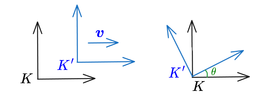
Where is the laboratory frame and is the moving frame with speed .
The inverse of the matrix is :
for -axis boost:
for general boost:
3.2.1 Velocity transformation
Suppose frame moves with velocity relative to frame along the positive x-axis. An object has velocity in frame and in frame , then the velocity transforms as:
If the boost is in an arbitrary direction *
Where represents the component of perpendicular to the boost direction. Assuming , *
3.2.2 The Proper Orthochronous Lorentz Group*
The Full Lorentz Group consists of all transformations that preserve the Minkowski metric. From the property above, it follows that . is a Lie group that possesses four disjoint, connected components. It can be expressed as the union of the Proper Orthochronous Lorentz Group (the identity component) and its cosets:
Infinitesimal Lorentz transformation
For infinite transformation ,
3.3 Tensor analysis (Minkowski spacetime)
3.3.1 4-description of vector / tensor
Primary 4-vector / tensor
4-velocity / accelerated velocity
Let to be the accelerated speed in the instantaneous co-moving frame and in the lab frame, one finds
4-momentum
4-force
Since ,
4-operator
Three fundamental invariant tensor in the Minkowski space
The recursion formula of decomposition
with base case is . for ex.,
Dual tensor of asymmetric matrix
Dual tensor of asymmetric matrix is
Eigenvalue equation of second-order tensors
the Principal Invariants
for an asymmetric matrix ,
4 Lagrangian Formulation of the EM Field
4.1 Covariant EM equation
4.1.1 Maxwell's equation
Electromagnetic Field Tensor
or simply
and two invariants
4-form Maxwell's equation
Differential 2-form of electromagnetic field tensor *
Gauge invariance
Thus, the field strength tensor remains invariant under the gauge transformation
4-form Maxwell's equation under the Lorenz gauge ,
4.1.2 Lorentz transformation of EM field
from Lorentz transformation of :
one finds
or more neatly (define ),
Electric-like / Magnetic-like / Light-like field
In the lab frame , if
and , in the inertial frame with speed . The cycloidal motion will transform into a hyperbolic motion.
and , in the inertial frame with speed , which is precisely the electric field drift velocity.
and , in the photon frame with speed (well, at present, this cannot be achieved).
, in the inertial frame with speed satisfy .
4.1.3 4-wave vector
4-form Wave equation for the field strength tensor can be derived from 4-form Maxwell's equation,
Thus, the monochromatic plane wave satisfies with the definition of 4-wave vector,
Lorentz transformation of . assuming ,
The relativistic Doppler formula demonstrates that whether the observer approaches the source or the source approaches the observer, as long as their relative velocity and the rest frequency of the source are identical, the observed frequency remains the same. This differs from the classical case; the observed frequency is always,
4.1.4 Conservation / Continuity equation
4-current & charge conservation
Define the 4-current,
Note: Since the total charge is a Lorentz invariant but the volume undergoes length contraction (), the charge density must increase by the same factor, .
Furthermore, while the time interval dilates () and the spatial volume element contracts (), these two factors exactly cancel each other out. This ensures that the four-dimensional spacetime volume is a Lorentz invariant (scalar).
The current's 4-divergence is zero,
A 4-vector is referred to as a conserved current if . The corresponding conserved charge, defined as , is a Lorentz invariant.
Mass conservation
Energy-momentum tensor conservation
4-Lorentz force
for single particle with charge , . thus,
Energy-momentum tensor of EM field
Energy-momentum tensor of particles
Energy-momentum conservation
or
relevant conserved charges are
Angular energy-momentum conservation*
4-angular momentum conservation
4-moment of force
relevant conserved charges are
The second term in the right side of is the velocity of total energy, which is proportional to , namely energy center moving in a straight line.
For the action , provided that the boundaries , are fixed and at the boundaries, then the principle of least action yields the Lagrange equation of particles as follows:
Gauge transformation
Covariant Lagrange equation for Relativistic Particle
For the action , provided that the endpoints are fixed and at the boundaries, then
Gauge transformation is .
Lagrange equation for Scalar Field
For the action , provided that the boundary of the spacetime region is fixed and on the boundary, then
Gauge transformation is .
Lagrange equation for Vector Field
For the action , provided that the boundary of the spacetime region is fixed and on the boundary, then
Gauge transformation is .
Generalized Lagrange Equation for Vector Field
For the action , provided that the boundary of the spacetime region is fixed, and the field variation along with its derivatives up to order vanish on the boundary (i.e., on for all ), then the generalized Euler-Lagrange equation reads,
Gauge transformation is .
4.2.2 Particles' motion
Substituting into the Lagrange equation yields and , respectively.
4.2.3 Field equation
Klein-Gordon field *
Substituting into the Lagrange equation yields Klein-Gordon equation , which has a monochromatic plane solution without the mass source , and
For a static, spherically symmetric source, the field equation reduces to . The physically meaningful solution (vanishing at infinity) is the Yukawa potential,
EM field
Substituting into the Lagrange equation yields the covariant Maxwell's equations with a source term,
4.3 Covariant single particle motion equation
4.3.1 Single particle in uniform electric field
Assuming and the particle is at rest and at time (at every subsequent moment , , and are parallel to ) . One finds
thus ,
This is a hyperbola, which can also be expressed in the form with the parameter . First above,
Since ,
and substituting into yields,
4.3.2 Single particle in uniform magnetic field
Assuming and the particle satisfies , , and at time . One finds
with relativistic cyclotron frequency , then integral
This depicts a spiral line moving along the axis. Since ,
with cyclotron radius and classic gyro-frequency .
4.3.3 Single particle in uniform electromagnetic field *
Perpendicular field
Assuming with , . Refer to 4-Lorentz force and Lorentz equation , One finds
Take the derivative of the second expression above with respect to the proper time ,
Substitute the 1-st and 3-rd equation into the above equation:
is a Lorentz invariant that we are all familiar with. Define , then the solutions fall into three categories:
Magnetic dominance
If , namely , the equation becomes the harmonic oscillator equation . However, it's complex to write out the parametric equations for the particle's motion in full. We adopt to a boost with since in the new inertial frame, with . 4-velocity component equation is simplified to
If , namely , the equation becomes the hyperbolic equation . Adopt to a boost with since in the new inertial frame, with . 4-velocity component equation is simplified to
If , namely , the equation becomes the light equation . 4-velocity component equation is simplified to
Thus
Then integral
Since
namely it's a particle propagating in the -direction at the speed of light as .
Non-Perpendicular field
If , one can find a inertial frame with the speed satisfying where . Therefore, Assuming with , , the solution is a spiral motion that undergoes hyperbolic acceleration in the direction.
4.4 Noether's theorem of field *
In this section, () denotes the components of a multicomponent field, but will be abbreviated as . When appears twice, it implies summation over .
4.4.1 Variation of field
Formal variation
Total variation
Relation of the two variation
4.4.2 Formal variation of Lagrangian
Since the field equation wouldn't change under the gauge , one find a conserved current / Noether current,
4.4.3 Total variation of Lagrangian
where the conserved current density is
or
Warning: the regular energy-momentum tensor is not symmetric generally not symmetric for fields with spin (such as the electromagnetic field with spin-1). An additional divergence term needs to be introduced to ensure symmetry (refer to Electrodynamics: 3. Symmetric correction).
Addition: Under the metric, conventionally , whereas for the , it's . This convention ensures that the energy density always satisfies the standard relation . Furthermore, the distinction between and its transposed counterpart amounts to a total divergence term (i.e., ). Consequently, serves as an equally valid alternative for describing the conserved currents.
4.4.4 Noether's theorem of field
Noether's theorem: If under the transformation , then is the conserved current satisfying
Space-time Translation
Consider a global infinitesimal translation . The field transforms as a scalar, hence . The Noether current is:
The conserved 4-momentum is,
needs to be corrected before we can obtain the physically meaningful expression of as well.
Rotations and Boosts
Consider an infinitesimal Lorentz transformation: , hence and ,